how to find what is the distribution of an attribute python

Statistics ( scipy.stats

Random variables

There are 2 general distribution classes that take been implemented for encapsulating continuous random variables and discrete random variables. Over lxxx continuous random variables (RVs) and 10 discrete random variables have been implemented using these classes. Also this, new routines and distributions tin can be hands added by the finish user. (If y'all create ane, please contribute it.)

All of the statistics functions are located in the sub-bundle scipy.stats and a adequately consummate listing of these functions can be obtained using info(stats) . The list of the random variables bachelor can too exist obtained from the docstring for the stats sub-bundle.

In the discussion below, we mostly focus on continuous RVs. Nearly everything also applies to detached variables, but we bespeak out some differences here: Specific points for discrete distributions.

In the code samples below, we assume that the scipy.stats package is imported as

                            >>>                            from              scipy              import              stats            

and in some cases we assume that individual objects are imported equally

                            >>>                            from              scipy.stats              import              norm            

Getting help

Starting time of all, all distributions are accompanied with help functions. To obtain just some basic information, we print the relevant docstring: print(stats.norm.__doc__) .

To discover the back up, i.due east., upper and lower bounds of the distribution, call:

                                >>>                                print                (                'premises of distribution lower:                                %s                , upper:                                %south                '                %                norm                .                back up                ())                bounds of distribution lower: -inf, upper: inf              

We can listing all methods and properties of the distribution with dir(norm) . As information technology turns out, some of the methods are private, although they are not named as such (their names practise not offset with a leading underscore), for case veccdf , are just available for internal calculation (those methods will give warnings when one tries to use them, and will be removed at some point).

To obtain the real chief methods, nosotros list the methods of the frozen distribution. (We explicate the pregnant of a frozen distribution beneath).

                                >>>                                rv                =                norm                ()                >>>                                dir                (                rv                )                # reformatted                ['__class__', '__delattr__', '__dict__', '__dir__', '__doc__', '__eq__',                                  '__format__', '__ge__', '__getattribute__', '__gt__', '__hash__',                                  '__init__', '__le__', '__lt__', '__module__', '__ne__', '__new__',                                  '__reduce__', '__reduce_ex__', '__repr__', '__setattr__', '__sizeof__',                                  '__str__', '__subclasshook__', '__weakref__', 'a', 'args', 'b', 'cdf',                                  'dist', 'entropy', 'expect', 'interval', 'isf', 'kwds', 'logcdf',                                  'logpdf', 'logpmf', 'logsf', 'mean', 'median', 'moment', 'pdf', 'pmf',                                  'ppf', 'random_state', 'rvs', 'sf', 'stats', 'std', 'var']              

Finally, we can obtain the listing of bachelor distribution through introspection:

                                >>>                                dist_continu                =                [                d                for                d                in                dir                (                stats                )                if                ...                                isinstance                (                getattr                (                stats                ,                d                ),                stats                .                rv_continuous                )]                >>>                                dist_discrete                =                [                d                for                d                in                dir                (                stats                )                if                ...                                isinstance                (                getattr                (                stats                ,                d                ),                stats                .                rv_discrete                )]                >>>                                print                (                'number of continuous distributions:                                %d                '                %                len                (                dist_continu                ))                number of continuous distributions: 104                >>>                                print                (                'number of detached distributions:                                %d                '                %                len                (                dist_discrete                ))                number of detached distributions:   19              

Common methods

The main public methods for continuous RVs are:

  • rvs: Random Variates

  • pdf: Probability Density Function

  • cdf: Cumulative Distribution Role

  • sf: Survival Function (1-CDF)

  • ppf: Percent Point Function (Changed of CDF)

  • isf: Inverse Survival Function (Inverse of SF)

  • stats: Return mean, variance, (Fisher'south) skew, or (Fisher's) kurtosis

  • moment: non-primal moments of the distribution

Allow'southward take a normal RV every bit an case.

To compute the cdf at a number of points, we can pass a list or a numpy assortment.

                                >>>                                norm                .                cdf                ([                -                1.                ,                0                ,                one                ])                array([ 0.15865525,  0.five,  0.84134475])                >>>                                import                numpy                as                np                >>>                                norm                .                cdf                (                np                .                array                ([                -                one.                ,                0                ,                i                ]))                assortment([ 0.15865525,  0.5,  0.84134475])              

Thus, the basic methods, such every bit pdf, cdf, and then on, are vectorized.

Other generally useful methods are supported besides:

                                >>>                                norm                .                mean                (),                norm                .                std                (),                norm                .                var                ()                (0.0, 1.0, i.0)                >>>                                norm                .                stats                (                moments                =                "mv"                )                (array(0.0), array(1.0))              

To find the median of a distribution, we tin use the percent point function ppf , which is the inverse of the cdf :

To generate a sequence of random variates, use the size keyword argument:

                                >>>                                norm                .                rvs                (                size                =                3                )                assortment([-0.35687759,  1.34347647, -0.11710531])   # random              

Don't recall that norm.rvs(v) generates 5 variates:

                                >>>                                norm                .                rvs                (                5                )                5.471435163732493  # random              

Here, 5 with no keyword is beingness interpreted as the commencement possible keyword argument, loc , which is the first of a pair of keyword arguments taken past all continuous distributions. This brings united states of america to the topic of the next subsection.

Random number generation

Cartoon random numbers relies on generators from numpy.random bundle. In the examples above, the specific stream of random numbers is not reproducible across runs. To accomplish reproducibility, y'all can explicitly seed a random number generator. In NumPy, a generator is an case of numpy.random.Generator . Here is the canonical mode to create a generator:

                                >>>                                from                numpy.random                import                default_rng                >>>                                rng                =                default_rng                ()              

And fixing the seed can exist done similar this:

                                >>>                                # do NOT copy this value                >>>                                rng                =                default_rng                (                301439351238479871608357552876690613766                )              

Warning

Do not use this number or common values such as 0. Using just a small gear up of seeds to instantiate larger state spaces means that there are some initial states that are incommunicable to reach. This creates some biases if everyone uses such values. A good way to get a seed is to use a numpy.random.SeedSequence :

                                    >>>                                    from                  numpy.random                  import                  SeedSequence                  >>>                                    print                  (                  SeedSequence                  ()                  .                  entropy                  )                  301439351238479871608357552876690613766  # random                

The random_state parameter in distributions accepts an instance of numpy.random.Generator class, or an integer, which is then used to seed an internal Generator object:

                                >>>                                norm                .                rvs                (                size                =                5                ,                random_state                =                rng                )                array([ 0.47143516, -1.19097569,  one.43270697, -0.3126519 , -0.72058873])  # random              

For further info, see NumPy'southward documentation.

To acquire more about the random number samplers implemented in SciPy, come across non-uniform random number sampling tutorial and quasi monte carlo tutorial

Shifting and scaling

All continuous distributions have loc and calibration as keyword parameters to adjust the location and scale of the distribution, e.g., for the standard normal distribution, the location is the mean and the scale is the standard departure.

                                >>>                                norm                .                stats                (                loc                =                three                ,                calibration                =                iv                ,                moments                =                "mv"                )                (array(iii.0), array(16.0))              

In many cases, the standardized distribution for a random variable X is obtained through the transformation (X - loc) / scale . The default values are loc = 0 and scale = ane .

Smart use of loc and scale can help modify the standard distributions in many ways. To illustrate the scaling farther, the cdf of an exponentially distributed RV with hateful \(ane/\lambda\) is given past

\[F(x) = 1 - \exp(-\lambda ten)\]

By applying the scaling rule above, it tin be seen that by taking calibration = i./lambda nosotros get the proper scale.

                                >>>                                from                scipy.stats                import                expon                >>>                                expon                .                mean                (                scale                =                3.                )                three.0              

Notation

Distributions that take shape parameters may crave more than simple application of loc and/or scale to achieve the desired form. For example, the distribution of two-D vector lengths given a constant vector of length \(R\) perturbed by independent N(0, \(\sigma^2\)) deviations in each component is rice(\(R/\sigma\), scale= \(\sigma\)). The first argument is a shape parameter that needs to be scaled forth with \(10\).

The uniform distribution is besides interesting:

                                >>>                                from                scipy.stats                import                uniform                >>>                                uniform                .                cdf                ([                0                ,                ane                ,                2                ,                iii                ,                4                ,                5                ],                loc                =                1                ,                scale                =                4                )                assortment([ 0.  ,  0.  ,  0.25,  0.five ,  0.75,  one.  ])              

Finally, recall from the previous paragraph that we are left with the problem of the meaning of norm.rvs(5) . As it turns out, calling a distribution like this, the first argument, i.e., the 5, gets passed to gear up the loc parameter. Permit's see:

                                >>>                                np                .                hateful                (                norm                .                rvs                (                v                ,                size                =                500                ))                5.0098355106969992  # random              

Thus, to explicate the output of the example of the last section: norm.rvs(5) generates a single ordinarily distributed random variate with hateful loc=5 , because of the default size=one .

We recommend that y'all gear up loc and scale parameters explicitly, past passing the values as keywords rather than as arguments. Repetition tin can be minimized when calling more than than one method of a given RV by using the technique of Freezing a Distribution, equally explained below.

Shape parameters

While a general continuous random variable tin can exist shifted and scaled with the loc and scale parameters, some distributions require additional shape parameters. For case, the gamma distribution with density

\[\gamma(ten, a) = \frac{\lambda (\lambda ten)^{a-1}}{\Gamma(a)} due east^{-\lambda ten}\;,\]

requires the shape parameter \(a\). Observe that setting \(\lambda\) can be obtained past setting the scale keyword to \(i/\lambda\).

Permit's check the number and name of the shape parameters of the gamma distribution. (We know from the above that this should exist 1.)

                                >>>                                from                scipy.stats                import                gamma                >>>                                gamma                .                numargs                1                >>>                                gamma                .                shapes                'a'              

Now, nosotros set the value of the shape variable to 1 to obtain the exponential distribution, so that nosotros compare easily whether nosotros get the results we expect.

                                >>>                                gamma                (                1                ,                scale                =                2.                )                .                stats                (                moments                =                "mv"                )                (array(2.0), array(4.0))              

Detect that we can also specify shape parameters as keywords:

                                >>>                                gamma                (                a                =                1                ,                calibration                =                two.                )                .                stats                (                moments                =                "mv"                )                (array(2.0), array(four.0))              

Freezing a distribution

Passing the loc and scale keywords time and again tin can become quite bothersome. The concept of freezing a RV is used to solve such problems.

                                >>>                                rv                =                gamma                (                i                ,                calibration                =                2.                )              

By using rv we no longer have to include the scale or the shape parameters anymore. Thus, distributions can exist used in one of ii means, either by passing all distribution parameters to each method telephone call (such equally we did earlier) or past freezing the parameters for the instance of the distribution. Let u.s. bank check this:

                                >>>                                rv                .                mean                (),                rv                .                std                ()                (two.0, 2.0)              

This is, indeed, what we should get.

Broadcasting

The bones methods pdf , so on, satisfy the usual numpy broadcasting rules. For example, nosotros tin summate the critical values for the upper tail of the t distribution for different probabilities and degrees of freedom.

                                >>>                                stats                .                t                .                isf                ([                0.i                ,                0.05                ,                0.01                ],                [[                10                ],                [                11                ]])                array([[ 1.37218364,  ane.81246112,  ii.76376946],                                  [ 1.36343032,  i.79588482,  2.71807918]])              

Here, the offset row contains the critical values for x degrees of freedom and the second row for 11 degrees of liberty (d.o.f.). Thus, the broadcasting rules give the same result of calling isf twice:

                                >>>                                stats                .                t                .                isf                ([                0.1                ,                0.05                ,                0.01                ],                10                )                array([ ane.37218364,  1.81246112,  2.76376946])                >>>                                stats                .                t                .                isf                ([                0.ane                ,                0.05                ,                0.01                ],                11                )                assortment([ 1.36343032,  1.79588482,  2.71807918])              

If the array with probabilities, i.e., [0.1, 0.05, 0.01] and the assortment of degrees of liberty i.e., [ten, xi, 12] , have the same array shape, then chemical element-wise matching is used. As an example, nosotros tin can obtain the 10% tail for 10 d.o.f., the 5% tail for 11 d.o.f. and the 1% tail for 12 d.o.f. by calling

                                >>>                                stats                .                t                .                isf                ([                0.1                ,                0.05                ,                0.01                ],                [                10                ,                11                ,                12                ])                array([ 1.37218364,  1.79588482,  two.68099799])              

Specific points for discrete distributions

Discrete distributions accept mostly the aforementioned bones methods as the continuous distributions. However pdf is replaced by the probability mass office pmf , no interpretation methods, such as fit, are available, and scale is not a valid keyword parameter. The location parameter, keyword loc , tin can still exist used to shift the distribution.

The computation of the cdf requires some actress attending. In the example of continuous distribution, the cumulative distribution part is, in most standard cases, strictly monotonic increasing in the premises (a,b) and has, therefore, a unique inverse. The cdf of a discrete distribution, even so, is a step function, hence the inverse cdf, i.e., the percent indicate part, requires a unlike definition:

                                ppf                (                q                )                =                min                {                x                :                cdf                (                x                )                >=                q                ,                ten                integer                }              

For further info, come across the docs here.

We tin await at the hypergeometric distribution every bit an example

                                >>>                                from                scipy.stats                import                hypergeom                >>>                                [                M                ,                north                ,                Due north                ]                =                [                20                ,                7                ,                12                ]              

If nosotros use the cdf at some integer points and then evaluate the ppf at those cdf values, we get the initial integers back, for example

                                >>>                                10                =                np                .                arange                (                4                )                *                2                >>>                                10                array([0, 2, 4, vi])                >>>                                prb                =                hypergeom                .                cdf                (                x                ,                M                ,                due north                ,                North                )                >>>                                prb                array([  1.03199174e-04,   5.21155831e-02,   vi.08359133e-01,                                  9.89783282e-01])                >>>                                hypergeom                .                ppf                (                prb                ,                M                ,                northward                ,                North                )                array([ 0.,  two.,  4.,  half dozen.])              

If we apply values that are not at the kinks of the cdf step function, we get the next higher integer back:

                                >>>                                hypergeom                .                ppf                (                prb                +                1e-eight                ,                M                ,                northward                ,                Due north                )                array([ 1.,  iii.,  five.,  7.])                >>>                                hypergeom                .                ppf                (                prb                -                1e-8                ,                M                ,                north                ,                Northward                )                array([ 0.,  2.,  4.,  half-dozen.])              

Fitting distributions

The main boosted methods of the not frozen distribution are related to the estimation of distribution parameters:

  • fit: maximum likelihood interpretation of distribution parameters, including location

    and scale

  • fit_loc_scale: interpretation of location and scale when shape parameters are given

  • nnlf: negative log likelihood office

  • wait: calculate the expectation of a function confronting the pdf or pmf

Performance issues and cautionary remarks

The functioning of the individual methods, in terms of speed, varies widely by distribution and method. The results of a method are obtained in i of two ways: either by explicit calculation, or by a generic algorithm that is independent of the specific distribution.

Explicit adding, on the ane manus, requires that the method is directly specified for the given distribution, either through analytic formulas or through special functions in scipy.special or numpy.random for rvs . These are commonly relatively fast calculations.

The generic methods, on the other paw, are used if the distribution does not specify any explicit calculation. To ascertain a distribution, only one of pdf or cdf is necessary; all other methods can be derived using numeric integration and root finding. Nevertheless, these indirect methods can exist very slow. As an example, rgh = stats.gausshyper.rvs(0.5, two, two, two, size=100) creates random variables in a very indirect way and takes nearly 19 seconds for 100 random variables on my reckoner, while one meg random variables from the standard normal or from the t distribution accept just above i 2d.

Remaining issues

The distributions in scipy.stats have recently been corrected and improved and gained a considerable test suite; however, a few issues remain:

  • The distributions take been tested over some range of parameters; however, in some corner ranges, a few wrong results may remain.

  • The maximum likelihood interpretation in fit does non work with default starting parameters for all distributions and the user needs to supply good starting parameters. Too, for some distribution using a maximum likelihood estimator might inherently non be the all-time choice.

Building specific distributions

The next examples shows how to build your ain distributions. Farther examples prove the usage of the distributions and some statistical tests.

Making a continuous distribution, i.due east., subclassing rv_continuous

Making continuous distributions is fairly elementary.

                                >>>                                from                scipy                import                stats                >>>                                grade                deterministic_gen                (                stats                .                rv_continuous                ):                ...                                def                _cdf                (                cocky                ,                ten                ):                ...                                return                np                .                where                (                x                <                0                ,                0.                ,                1.                )                ...                                def                _stats                (                cocky                ):                ...                                render                0.                ,                0.                ,                0.                ,                0.              
                                >>>                                deterministic                =                deterministic_gen                (                name                =                "deterministic"                )                >>>                                deterministic                .                cdf                (                np                .                arange                (                -                3                ,                3                ,                0.5                ))                array([ 0.,  0.,  0.,  0.,  0.,  0.,  1.,  1.,  1.,  1.,  1.,  1.])              

Interestingly, the pdf is at present computed automatically:

                                >>>                                deterministic                .                pdf                (                np                .                arange                (                -                3                ,                3                ,                0.5                ))                array([  0.00000000e+00,   0.00000000e+00,   0.00000000e+00,                                  0.00000000e+00,   0.00000000e+00,   0.00000000e+00,                                  v.83333333e+04,   4.16333634e-12,   4.16333634e-12,                                  4.16333634e-12,   iv.16333634e-12,   four.16333634e-12])              

Exist aware of the functioning issues mentioned in Performance issues and cautionary remarks. The computation of unspecified common methods can become very slow, since only general methods are chosen, which, by their very nature, cannot employ whatsoever specific data nigh the distribution. Thus, as a cautionary example:

                                >>>                                from                scipy.integrate                import                quad                >>>                                quad                (                deterministic                .                pdf                ,                -                1e-one                ,                1e-1                )                (4.163336342344337e-xiii, 0.0)              

But this is not correct: the integral over this pdf should be one. Allow'southward make the integration interval smaller:

                                >>>                                quad                (                deterministic                .                pdf                ,                -                1e-3                ,                1e-3                )                # alert removed                (ane.000076872229173, 0.0010625571718182458)              

This looks improve. However, the problem originated from the fact that the pdf is not specified in the form definition of the deterministic distribution.

Subclassing rv_discrete

In the following, nosotros use stats.rv_discrete to generate a discrete distribution that has the probabilities of the truncated normal for the intervals centered effectually the integers.

General info

From the docstring of rv_discrete, help(stats.rv_discrete) ,

"You tin construct an capricious discrete rv where P{X=xk} = pk by passing to the rv_discrete initialization method (through the values= keyword) a tuple of sequences (xk, pk) which describes simply those values of 10 (xk) that occur with nonzero probability (pk)."

Next to this, at that place are some further requirements for this approach to work:

  • The keyword name is required.

  • The back up points of the distribution xk have to be integers.

  • The number of significant digits (decimals) needs to be specified.

In fact, if the last two requirements are not satisfied, an exception may be raised or the resulting numbers may exist incorrect.

An case

Permit's do the work. Outset:

                                >>>                                npoints                =                20                # number of integer support points of the distribution minus 1                >>>                                npointsh                =                npoints                //                2                >>>                                npointsf                =                float                (                npoints                )                >>>                                nbound                =                iv                # bounds for the truncated normal                >>>                                normbound                =                (                1                +                1                /                npointsf                )                *                nbound                # actual bounds of truncated normal                >>>                                grid                =                np                .                arange                (                -                npointsh                ,                npointsh                +                2                ,                1                )                # integer grid                >>>                                gridlimitsnorm                =                (                grid                -                0.five                )                /                npointsh                *                nbound                # bin limits for the truncnorm                >>>                                gridlimits                =                grid                -                0.v                # used later in the analysis                >>>                                grid                =                grid                [:                -                1                ]                >>>                                probs                =                np                .                diff                (                stats                .                truncnorm                .                cdf                (                gridlimitsnorm                ,                -                normbound                ,                normbound                ))                >>>                                gridint                =                grid              

And, finally, we can bracket rv_discrete :

                                >>>                                normdiscrete                =                stats                .                rv_discrete                (                values                =                (                gridint                ,                ...                                np                .                round                (                probs                ,                decimals                =                7                )),                name                =                'normdiscrete'                )              

Now that we have defined the distribution, nosotros have access to all common methods of discrete distributions.

                                >>>                                print                (                'mean =                                %6.4f                , variance =                                %half-dozen.4f                , skew =                                %six.4f                , kurtosis =                                %vi.4f                '                %                ...                                normdiscrete                .                stats                (                moments                =                'mvsk'                ))                hateful = -0.0000, variance = 6.3302, skew = 0.0000, kurtosis = -0.0076              
                                >>>                                nd_std                =                np                .                sqrt                (                normdiscrete                .                stats                (                moments                =                'v'                ))              

Testing the implementation

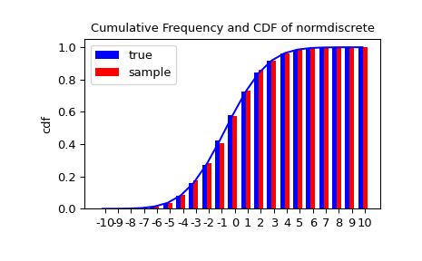
Let'southward generate a random sample and compare observed frequencies with the probabilities.

                                >>>                                n_sample                =                500                >>>                                rvs                =                normdiscrete                .                rvs                (                size                =                n_sample                )                >>>                                f                ,                l                =                np                .                histogram                (                rvs                ,                bins                =                gridlimits                )                >>>                                sfreq                =                np                .                vstack                ([                gridint                ,                f                ,                probs                *                n_sample                ])                .                T                >>>                                print                (                sfreq                )                [[-i.00000000e+01  0.00000000e+00  2.95019349e-02]  # random                                  [-9.00000000e+00  0.00000000e+00  ane.32294142e-01]                                  [-8.00000000e+00  0.00000000e+00  5.06497902e-01]                                  [-7.00000000e+00  two.00000000e+00  1.65568919e+00]                                  [-6.00000000e+00  1.00000000e+00  4.62125309e+00]                                  [-5.00000000e+00  9.00000000e+00  1.10137298e+01]                                  [-iv.00000000e+00  2.60000000e+01  2.24137683e+01]                                  [-three.00000000e+00  3.70000000e+01  iii.89503370e+01]                                  [-two.00000000e+00  5.10000000e+01  5.78004747e+01]                                  [-1.00000000e+00  vii.10000000e+01  7.32455414e+01]                                  [ 0.00000000e+00  7.40000000e+01  7.92618251e+01]                                  [ 1.00000000e+00  viii.90000000e+01  7.32455414e+01]                                  [ ii.00000000e+00  5.50000000e+01  5.78004747e+01]                                  [ iii.00000000e+00  5.00000000e+01  3.89503370e+01]                                  [ 4.00000000e+00  1.70000000e+01  2.24137683e+01]                                  [ v.00000000e+00  ane.10000000e+01  1.10137298e+01]                                  [ 6.00000000e+00  4.00000000e+00  4.62125309e+00]                                  [ 7.00000000e+00  3.00000000e+00  1.65568919e+00]                                  [ 8.00000000e+00  0.00000000e+00  v.06497902e-01]                                  [ 9.00000000e+00  0.00000000e+00  1.32294142e-01]                                  [ 1.00000000e+01  0.00000000e+00  2.95019349e-02]]              

../_images/normdiscr_plot1.png

../_images/normdiscr_plot2.png

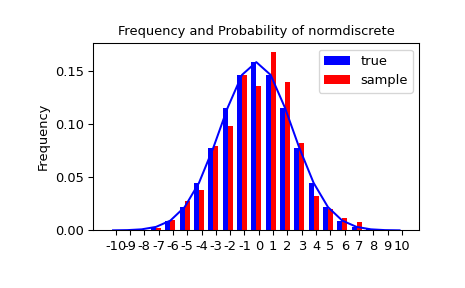
Next, nosotros can test whether our sample was generated past our norm-detached distribution. This likewise verifies whether the random numbers were generated correctly.

The chisquare test requires that at that place are a minimum number of observations in each bin. We combine the tail bins into larger bins and so that they contain enough observations.

                                >>>                                f2                =                np                .                hstack                ([                f                [:                5                ]                .                sum                (),                f                [                v                :                -                five                ],                f                [                -                5                :]                .                sum                ()])                >>>                                p2                =                np                .                hstack                ([                probs                [:                five                ]                .                sum                (),                probs                [                5                :                -                five                ],                probs                [                -                5                :]                .                sum                ()])                >>>                                ch2                ,                pval                =                stats                .                chisquare                (                f2                ,                p2                *                n_sample                )              
                                >>>                                print                (                'chisquare for normdiscrete: chi2 =                                %six.3f                                  pvalue =                                %6.4f                '                %                (                ch2                ,                pval                ))                chisquare for normdiscrete: chi2 = 12.466 pvalue = 0.4090  # random              

The pvalue in this case is high, so we can be quite confident that our random sample was actually generated by the distribution.

Analysing one sample

Outset, we create some random variables. We set a seed so that in each run nosotros get identical results to expect at. As an example we take a sample from the Student t distribution:

                            >>>                            x              =              stats              .              t              .              rvs              (              x              ,              size              =              one thousand              )            

Here, we prepare the required shape parameter of the t distribution, which in statistics corresponds to the degrees of liberty, to 10. Using size=1000 means that our sample consists of 1000 independently fatigued (pseudo) random numbers. Since we did not specify the keyword arguments loc and scale, those are fix to their default values zip and i.

Descriptive statistics

x is a numpy array, and nosotros take direct admission to all array methods, due east.g.,

                                >>>                                print                (                x                .                min                ())                # equivalent to np.min(10)                -three.78975572422  # random                >>>                                print                (                x                .                max                ())                # equivalent to np.max(x)                5.26327732981  # random                >>>                                print                (                x                .                mean                ())                # equivalent to np.mean(ten)                0.0140610663985  # random                >>>                                print                (                ten                .                var                ())                # equivalent to np.var(ten))                1.28899386208  # random              

How do the sample properties compare to their theoretical counterparts?

                                >>>                                chiliad                ,                v                ,                southward                ,                m                =                stats                .                t                .                stats                (                x                ,                moments                =                'mvsk'                )                >>>                                due north                ,                (                smin                ,                smax                ),                sm                ,                sv                ,                ss                ,                sk                =                stats                .                depict                (                x                )              
                                >>>                                sstr                =                '                %-14s                                  mean =                                %6.4f                , variance =                                %six.4f                , skew =                                %6.4f                , kurtosis =                                %half-dozen.4f                '                >>>                                print                (                sstr                %                (                'distribution:'                ,                m                ,                five                ,                s                ,                g                ))                distribution:  mean = 0.0000, variance = one.2500, skew = 0.0000, kurtosis = 1.0000  # random                >>>                                print                (                sstr                %                (                'sample:'                ,                sm                ,                sv                ,                ss                ,                sk                ))                sample:        mean = 0.0141, variance = ane.2903, skew = 0.2165, kurtosis = i.0556  # random              

Annotation: stats.describe uses the unbiased estimator for the variance, while np.var is the biased estimator.

For our sample the sample statistics differ a by a small amount from their theoretical counterparts.

T-examination and KS-examination

We can use the t-test to examination whether the mean of our sample differs in a statistically significant way from the theoretical expectation.

                                >>>                                print                (                't-statistic =                                %six.3f                                  pvalue =                                %6.4f                '                %                stats                .                ttest_1samp                (                ten                ,                m                ))                t-statistic =  0.391 pvalue = 0.6955  # random              

The pvalue is 0.7, this means that with an alpha fault of, for example, x%, we cannot reject the hypothesis that the sample mean is equal to cypher, the expectation of the standard t-distribution.

As an exercise, we can calculate our ttest also directly without using the provided role, which should requite us the aforementioned reply, and so it does:

                                >>>                                tt                =                (                sm                -                1000                )                /                np                .                sqrt                (                sv                /                float                (                n                ))                # t-statistic for mean                >>>                                pval                =                stats                .                t                .                sf                (                np                .                abs                (                tt                ),                n                -                one                )                *                2                # 2-sided pvalue = Prob(abs(t)>tt)                >>>                                impress                (                't-statistic =                                %half dozen.3f                                  pvalue =                                %vi.4f                '                %                (                tt                ,                pval                ))                t-statistic =  0.391 pvalue = 0.6955  # random              

The Kolmogorov-Smirnov test can be used to test the hypothesis that the sample comes from the standard t-distribution

                                >>>                                print                (                'KS-statistic D =                                %six.3f                                  pvalue =                                %half dozen.4f                '                %                stats                .                kstest                (                x                ,                't'                ,                (                ten                ,)))                KS-statistic D =  0.016 pvalue = 0.9571  # random              

Again, the p-value is high enough that nosotros cannot pass up the hypothesis that the random sample really is distributed according to the t-distribution. In existent applications, nosotros don't know what the underlying distribution is. If we perform the Kolmogorov-Smirnov examination of our sample against the standard normal distribution, and so we likewise cannot reject the hypothesis that our sample was generated by the normal distribution given that, in this example, the p-value is nigh 40%.

                                >>>                                print                (                'KS-statistic D =                                %6.3f                                  pvalue =                                %6.4f                '                %                stats                .                kstest                (                10                ,                'norm'                ))                KS-statistic D =  0.028 pvalue = 0.3918  # random              

Nonetheless, the standard normal distribution has a variance of 1, while our sample has a variance of 1.29. If we standardize our sample and examination it against the normal distribution, then the p-value is again big enough that nosotros cannot reject the hypothesis that the sample came grade the normal distribution.

                                >>>                                d                ,                pval                =                stats                .                kstest                ((                x                -                10                .                mean                ())                /                10                .                std                (),                'norm'                )                >>>                                impress                (                'KS-statistic D =                                %6.3f                                  pvalue =                                %6.4f                '                %                (                d                ,                pval                ))                KS-statistic D =  0.032 pvalue = 0.2397  # random              

Note: The Kolmogorov-Smirnov test assumes that we test against a distribution with given parameters, since, in the last case, nosotros estimated mean and variance, this assumption is violated and the distribution of the test statistic, on which the p-value is based, is not correct.

Tails of the distribution

Finally, we can check the upper tail of the distribution. We tin use the percent indicate function ppf, which is the inverse of the cdf role, to obtain the critical values, or, more directly, we can apply the inverse of the survival role

                                >>>                                crit01                ,                crit05                ,                crit10                =                stats                .                t                .                ppf                ([                i                -                0.01                ,                1                -                0.05                ,                one                -                0.10                ],                10                )                >>>                                print                (                'critical values from ppf at 1                %%                , five                %%                                  and x                %%                                                %8.4f                                                %8.4f                                                %viii.4f                '                %                (                crit01                ,                crit05                ,                crit10                ))                critical values from ppf at 1%, 5% and x%   2.7638   i.8125   i.3722                >>>                                print                (                'critical values from isf at one                %%                , 5                %%                                  and 10                %%                                                %8.4f                                                %eight.4f                                                %8.4f                '                %                tuple                (                stats                .                t                .                isf                ([                0.01                ,                0.05                ,                0.10                ],                10                )))                critical values from isf at one%, v% and 10%   ii.7638   one.8125   1.3722              
                                >>>                                freq01                =                np                .                sum                (                ten                >                crit01                )                /                float                (                n                )                *                100                >>>                                freq05                =                np                .                sum                (                x                >                crit05                )                /                float                (                n                )                *                100                >>>                                freq10                =                np                .                sum                (                x                >                crit10                )                /                bladder                (                due north                )                *                100                >>>                                print                (                'sample                                %%                -frequency at ane                %%                , 5                %%                                  and x                %%                                  tail                                %8.4f                                                %8.4f                                                %viii.4f                '                %                (                freq01                ,                freq05                ,                freq10                ))                sample %-frequency at one%, 5% and ten% tail   one.4000   5.8000  10.5000  # random              

In all iii cases, our sample has more weight in the top tail than the underlying distribution. Nosotros tin can briefly check a larger sample to come across if we get a closer match. In this example, the empirical frequency is quite close to the theoretical probability, merely if we repeat this several times, the fluctuations are still pretty large.

                                >>>                                freq05l                =                np                .                sum                (                stats                .                t                .                rvs                (                10                ,                size                =                10000                )                >                crit05                )                /                10000.0                *                100                >>>                                print                (                'larger sample                                %%                -frequency at 5                %%                                  tail                                %8.4f                '                %                freq05l                )                larger sample %-frequency at 5% tail   4.8000  # random              

We tin as well compare it with the tail of the normal distribution, which has less weight in the tails:

                                >>>                                print                (                'tail prob. of normal at i                %%                , 5                %%                                  and 10                %%                                                %viii.4f                                                %8.4f                                                %8.4f                '                %                ...                                tuple                (                stats                .                norm                .                sf                ([                crit01                ,                crit05                ,                crit10                ])                *                100                ))                tail prob. of normal at 1%, 5% and 10%   0.2857   3.4957   8.5003              

The chisquare examination can be used to test whether for a finite number of bins, the observed frequencies differ significantly from the probabilities of the hypothesized distribution.

                                >>>                                quantiles                =                [                0.0                ,                0.01                ,                0.05                ,                0.1                ,                1                -                0.10                ,                1                -                0.05                ,                i                -                0.01                ,                1.0                ]                >>>                                crit                =                stats                .                t                .                ppf                (                quantiles                ,                ten                )                >>>                                crit                array([       -inf, -ii.76376946, -1.81246112, -1.37218364,  1.37218364,                                  i.81246112,  2.76376946,         inf])                >>>                                n_sample                =                ten                .                size                >>>                                freqcount                =                np                .                histogram                (                10                ,                bins                =                crit                )[                0                ]                >>>                                tprob                =                np                .                unequal                (                quantiles                )                >>>                                nprob                =                np                .                diff                (                stats                .                norm                .                cdf                (                crit                ))                >>>                                tch                ,                tpval                =                stats                .                chisquare                (                freqcount                ,                tprob                *                n_sample                )                >>>                                nch                ,                npval                =                stats                .                chisquare                (                freqcount                ,                nprob                *                n_sample                )                >>>                                print                (                'chisquare for t:      chi2 =                                %half dozen.2f                                  pvalue =                                %half-dozen.4f                '                %                (                tch                ,                tpval                ))                chisquare for t:      chi2 =  2.30 pvalue = 0.8901  # random                >>>                                print                (                'chisquare for normal: chi2 =                                %6.2f                                  pvalue =                                %6.4f                '                %                (                nch                ,                npval                ))                chisquare for normal: chi2 = 64.lx pvalue = 0.0000  # random              

We see that the standard normal distribution is clearly rejected, while the standard t-distribution cannot be rejected. Since the variance of our sample differs from both standard distributions, we can over again redo the test taking the estimate for calibration and location into account.

The fit method of the distributions can be used to estimate the parameters of the distribution, and the exam is repeated using probabilities of the estimated distribution.

                                >>>                                tdof                ,                tloc                ,                tscale                =                stats                .                t                .                fit                (                x                )                >>>                                nloc                ,                nscale                =                stats                .                norm                .                fit                (                x                )                >>>                                tprob                =                np                .                diff                (                stats                .                t                .                cdf                (                crit                ,                tdof                ,                loc                =                tloc                ,                scale                =                tscale                ))                >>>                                nprob                =                np                .                diff                (                stats                .                norm                .                cdf                (                crit                ,                loc                =                nloc                ,                scale                =                nscale                ))                >>>                                tch                ,                tpval                =                stats                .                chisquare                (                freqcount                ,                tprob                *                n_sample                )                >>>                                nch                ,                npval                =                stats                .                chisquare                (                freqcount                ,                nprob                *                n_sample                )                >>>                                print                (                'chisquare for t:      chi2 =                                %vi.2f                                  pvalue =                                %6.4f                '                %                (                tch                ,                tpval                ))                chisquare for t:      chi2 =  1.58 pvalue = 0.9542  # random                >>>                                print                (                'chisquare for normal: chi2 =                                %six.2f                                  pvalue =                                %6.4f                '                %                (                nch                ,                npval                ))                chisquare for normal: chi2 = 11.08 pvalue = 0.0858  # random              

Taking account of the estimated parameters, we tin can still reject the hypothesis that our sample came from a normal distribution (at the 5% level), merely again, with a p-value of 0.95, nosotros cannot pass up the t-distribution.

Special tests for normal distributions

Since the normal distribution is the most mutual distribution in statistics, there are several additional functions available to examination whether a sample could have been drawn from a normal distribution.

Outset, we tin test if skew and kurtosis of our sample differ significantly from those of a normal distribution:

                                >>>                                print                (                'normal skewtest teststat =                                %six.3f                                  pvalue =                                %6.4f                '                %                stats                .                skewtest                (                x                ))                normal skewtest teststat =  2.785 pvalue = 0.0054  # random                >>>                                print                (                'normal kurtosistest teststat =                                %6.3f                                  pvalue =                                %half dozen.4f                '                %                stats                .                kurtosistest                (                ten                ))                normal kurtosistest teststat =  4.757 pvalue = 0.0000  # random              

These two tests are combined in the normality test

                                >>>                                impress                (                'normaltest teststat =                                %6.3f                                  pvalue =                                %half dozen.4f                '                %                stats                .                normaltest                (                x                ))                normaltest teststat = 30.379 pvalue = 0.0000  # random              

In all three tests, the p-values are very low and we can reject the hypothesis that the our sample has skew and kurtosis of the normal distribution.

Since skew and kurtosis of our sample are based on central moments, we go exactly the same results if we test the standardized sample:

                                >>>                                impress                (                'normaltest teststat =                                %6.3f                                  pvalue =                                %6.4f                '                %                ...                                stats                .                normaltest                ((                10                -                ten                .                mean                ())                /                x                .                std                ()))                normaltest teststat = 30.379 pvalue = 0.0000  # random              

Because normality is rejected then strongly, nosotros tin check whether the normaltest gives reasonable results for other cases:

                                >>>                                print                (                'normaltest teststat =                                %6.3f                                  pvalue =                                %vi.4f                '                %                ...                                stats                .                normaltest                (                stats                .                t                .                rvs                (                x                ,                size                =                100                )))                normaltest teststat =  4.698 pvalue = 0.0955  # random                >>>                                impress                (                'normaltest teststat =                                %6.3f                                  pvalue =                                %6.4f                '                %                ...                                stats                .                normaltest                (                stats                .                norm                .                rvs                (                size                =                1000                )))                normaltest teststat =  0.613 pvalue = 0.7361  # random              

When testing for normality of a small sample of t-distributed observations and a large sample of normal-distributed observations, then in neither case can we reject the null hypothesis that the sample comes from a normal distribution. In the first case, this is because the test is not powerful enough to distinguish a t and a normally distributed random variable in a small sample.

Comparison two samples

In the following, we are given two samples, which can come either from the aforementioned or from dissimilar distribution, and we want to test whether these samples take the same statistical properties.

Comparing means

Test with sample with identical ways:

                                >>>                                rvs1                =                stats                .                norm                .                rvs                (                loc                =                5                ,                calibration                =                10                ,                size                =                500                )                >>>                                rvs2                =                stats                .                norm                .                rvs                (                loc                =                v                ,                scale                =                ten                ,                size                =                500                )                >>>                                stats                .                ttest_ind                (                rvs1                ,                rvs2                )                Ttest_indResult(statistic=-0.5489036175088705, pvalue=0.5831943748663959)  # random              

Test with sample with unlike means:

                                >>>                                rvs3                =                stats                .                norm                .                rvs                (                loc                =                8                ,                scale                =                10                ,                size                =                500                )                >>>                                stats                .                ttest_ind                (                rvs1                ,                rvs3                )                Ttest_indResult(statistic=-iv.533414290175026, pvalue=six.507128186389019e-06)  # random              

Kolmogorov-Smirnov exam for two samples ks_2samp

For the instance, where both samples are drawn from the aforementioned distribution, we cannot reject the null hypothesis, since the pvalue is high

                                >>>                                stats                .                ks_2samp                (                rvs1                ,                rvs2                )                KstestResult(statistic=0.026, pvalue=0.9959527565364388)  # random              

In the second example, with different location, i.eastward., means, nosotros can reject the zero hypothesis, since the pvalue is beneath 1%

                                >>>                                stats                .                ks_2samp                (                rvs1                ,                rvs3                )                KstestResult(statistic=0.114, pvalue=0.00299005061044668)  # random              

Kernel density estimation

A common chore in statistics is to guess the probability density part (PDF) of a random variable from a set of data samples. This task is chosen density estimation. The well-nigh well-known tool to practice this is the histogram. A histogram is a useful tool for visualization (mainly considering everyone understands information technology), but doesn't employ the available data very efficiently. Kernel density estimation (KDE) is a more efficient tool for the same task. The gaussian_kde computer can exist used to estimate the PDF of univariate as well as multivariate information. It works all-time if the data is unimodal.

Univariate interpretation

We first with a minimal amount of data in order to see how gaussian_kde works and what the different options for bandwidth choice do. The data sampled from the PDF are shown as blue dashes at the bottom of the figure (this is called a rug plot):

                                >>>                                from                scipy                import                stats                >>>                                import                matplotlib.pyplot                as                plt              
                                >>>                                x1                =                np                .                array                ([                -                7                ,                -                5                ,                1                ,                four                ,                5                ],                dtype                =                np                .                float64                )                >>>                                kde1                =                stats                .                gaussian_kde                (                x1                )                >>>                                kde2                =                stats                .                gaussian_kde                (                x1                ,                bw_method                =                'silverman'                )              
                                >>>                                fig                =                plt                .                figure                ()                >>>                                ax                =                fig                .                add_subplot                (                111                )              
                                >>>                                ax                .                plot                (                x1                ,                np                .                zeros                (                x1                .                shape                ),                'b+'                ,                ms                =                twenty                )                # rug plot                >>>                                x_eval                =                np                .                linspace                (                -                10                ,                10                ,                num                =                200                )                >>>                                ax                .                plot                (                x_eval                ,                kde1                (                x_eval                ),                'yard-'                ,                label                =                "Scott's Rule"                )                >>>                                ax                .                plot                (                x_eval                ,                kde2                (                x_eval                ),                'r-'                ,                label                =                "Silverman's Dominion"                )              

../_images/stats-1.png

We meet that there is very little difference between Scott'due south Dominion and Silverman'due south Rule, and that the bandwidth selection with a limited amount of data is probably a bit too wide. We can define our ain bandwidth part to get a less smoothed-out result.

                                >>>                                def                my_kde_bandwidth                (                obj                ,                fac                =                1.                /                5                ):                ...                                """We utilise Scott's Rule, multiplied past a constant cistron."""                ...                                render                np                .                power                (                obj                .                n                ,                -                1.                /                (                obj                .                d                +                four                ))                *                fac              
                                >>>                                fig                =                plt                .                effigy                ()                >>>                                ax                =                fig                .                add_subplot                (                111                )              
                                >>>                                ax                .                plot                (                x1                ,                np                .                zeros                (                x1                .                shape                ),                'b+'                ,                ms                =                twenty                )                # rug plot                >>>                                kde3                =                stats                .                gaussian_kde                (                x1                ,                bw_method                =                my_kde_bandwidth                )                >>>                                ax                .                plot                (                x_eval                ,                kde3                (                x_eval                ),                'thousand-'                ,                characterization                =                "With smaller BW"                )              

../_images/kde_plot2.png

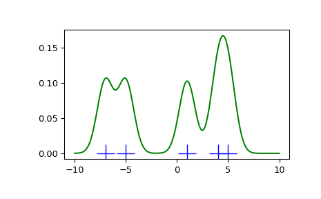
We see that if we set bandwidth to be very narrow, the obtained approximate for the probability density function (PDF) is just the sum of Gaussians around each data point.

Nosotros now take a more than realistic example and look at the departure between the two available bandwidth pick rules. Those rules are known to work well for (shut to) normal distributions, but even for unimodal distributions that are quite strongly non-normal they work reasonably well. As a not-normal distribution we take a Student's T distribution with 5 degrees of freedom.

                                import                numpy                as                np                import                matplotlib.pyplot                as                plt                from                scipy                import                stats                rng                =                np                .                random                .                default_rng                ()                x1                =                rng                .                normal                (                size                =                200                )                # random data, normal distribution                xs                =                np                .                linspace                (                x1                .                min                ()                -                one                ,                x1                .                max                ()                +                1                ,                200                )                kde1                =                stats                .                gaussian_kde                (                x1                )                kde2                =                stats                .                gaussian_kde                (                x1                ,                bw_method                =                'silverman'                )                fig                =                plt                .                figure                (                figsize                =                (                8                ,                half-dozen                ))                ax1                =                fig                .                add_subplot                (                211                )                ax1                .                plot                (                x1                ,                np                .                zeros                (                x1                .                shape                ),                'b+'                ,                ms                =                12                )                # rug plot                ax1                .                plot                (                xs                ,                kde1                (                xs                ),                'k-'                ,                label                =                "Scott's Rule"                )                ax1                .                plot                (                xs                ,                kde2                (                xs                ),                'b-'                ,                label                =                "Silverman's Dominion"                )                ax1                .                plot                (                xs                ,                stats                .                norm                .                pdf                (                xs                ),                'r--'                ,                characterization                =                "True PDF"                )                ax1                .                set_xlabel                (                'x'                )                ax1                .                set_ylabel                (                'Density'                )                ax1                .                set_title                (                "Normal (peak) and Student'due south T$_{df=5}$ (bottom) distributions"                )                ax1                .                fable                (                loc                =                1                )                x2                =                stats                .                t                .                rvs                (                5                ,                size                =                200                ,                random_state                =                rng                )                # random data, T distribution                xs                =                np                .                linspace                (                x2                .                min                ()                -                1                ,                x2                .                max                ()                +                1                ,                200                )                kde3                =                stats                .                gaussian_kde                (                x2                )                kde4                =                stats                .                gaussian_kde                (                x2                ,                bw_method                =                'silverman'                )                ax2                =                fig                .                add_subplot                (                212                )                ax2                .                plot                (                x2                ,                np                .                zeros                (                x2                .                shape                ),                'b+'                ,                ms                =                12                )                # rug plot                ax2                .                plot                (                xs                ,                kde3                (                xs                ),                'k-'                ,                label                =                "Scott'southward Rule"                )                ax2                .                plot                (                xs                ,                kde4                (                xs                ),                'b-'                ,                label                =                "Silverman'south Dominion"                )                ax2                .                plot                (                xs                ,                stats                .                t                .                pdf                (                xs                ,                v                ),                'r--'                ,                label                =                "True PDF"                )                ax2                .                set_xlabel                (                'x'                )                ax2                .                set_ylabel                (                'Density'                )                plt                .                prove                ()              

../_images/kde_plot3.png

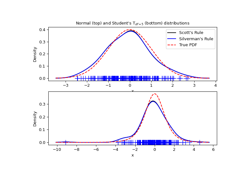
Nosotros now take a expect at a bimodal distribution with ane wider and one narrower Gaussian feature. We expect that this will be a more hard density to approximate, due to the different bandwidths required to accurately resolve each feature.

                                >>>                                from                functools                import                partial              
                                >>>                                loc1                ,                scale1                ,                size1                =                (                -                2                ,                1                ,                175                )                >>>                                loc2                ,                scale2                ,                size2                =                (                2                ,                0.2                ,                50                )                >>>                                x2                =                np                .                concatenate                ([                np                .                random                .                normal                (                loc                =                loc1                ,                scale                =                scale1                ,                size                =                size1                ),                ...                                np                .                random                .                normal                (                loc                =                loc2                ,                scale                =                scale2                ,                size                =                size2                )])              
                                >>>                                x_eval                =                np                .                linspace                (                x2                .                min                ()                -                1                ,                x2                .                max                ()                +                1                ,                500                )              
                                >>>                                kde                =                stats                .                gaussian_kde                (                x2                )                >>>                                kde2                =                stats                .                gaussian_kde                (                x2                ,                bw_method                =                'silverman'                )                >>>                                kde3                =                stats                .                gaussian_kde                (                x2                ,                bw_method                =                partial                (                my_kde_bandwidth                ,                fac                =                0.2                ))                >>>                                kde4                =                stats                .                gaussian_kde                (                x2                ,                bw_method                =                partial                (                my_kde_bandwidth                ,                fac                =                0.5                ))              
                                >>>                                pdf                =                stats                .                norm                .                pdf                >>>                                bimodal_pdf                =                pdf                (                x_eval                ,                loc                =                loc1                ,                scale                =                scale1                )                *                bladder                (                size1                )                /                x2                .                size                +                \                ...                                pdf                (                x_eval                ,                loc                =                loc2                ,                scale                =                scale2                )                *                float                (                size2                )                /                x2                .                size              
                                >>>                                fig                =                plt                .                effigy                (                figsize                =                (                8                ,                6                ))                >>>                                ax                =                fig                .                add_subplot                (                111                )              
                                >>>                                ax                .                plot                (                x2                ,                np                .                zeros                (                x2                .                shape                ),                'b+'                ,                ms                =                12                )                >>>                                ax                .                plot                (                x_eval                ,                kde                (                x_eval                ),                'thou-'                ,                label                =                "Scott's Rule"                )                >>>                                ax                .                plot                (                x_eval                ,                kde2                (                x_eval                ),                'b-'                ,                label                =                "Silverman's Rule"                )                >>>                                ax                .                plot                (                x_eval                ,                kde3                (                x_eval                ),                'one thousand-'                ,                label                =                "Scott * 0.2"                )                >>>                                ax                .                plot                (                x_eval                ,                kde4                (                x_eval                ),                'c-'                ,                label                =                "Scott * 0.5"                )                >>>                                ax                .                plot                (                x_eval                ,                bimodal_pdf                ,                'r--'                ,                label                =                "Bodily PDF"                )              
                                >>>                                ax                .                set_xlim                ([                x_eval                .                min                (),                x_eval                .                max                ()])                >>>                                ax                .                fable                (                loc                =                2                )                >>>                                ax                .                set_xlabel                (                'ten'                )                >>>                                ax                .                set_ylabel                (                'Density'                )                >>>                                plt                .                show                ()              

../_images/kde_plot4.png

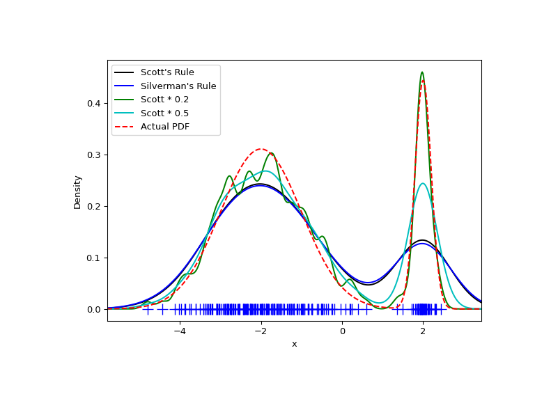
Every bit expected, the KDE is not as shut to the true PDF as we would like due to the unlike characteristic size of the two features of the bimodal distribution. Past halving the default bandwidth ( Scott * 0.5 ), nosotros tin practice somewhat better, while using a gene 5 smaller bandwidth than the default doesn't smooth enough. What we really need, though, in this case, is a non-compatible (adaptive) bandwidth.

Multivariate estimation

With gaussian_kde we tin perform multivariate, as well as univariate estimation. We demonstrate the bivariate case. Kickoff, we generate some random data with a model in which the two variates are correlated.

                                >>>                                def                mensurate                (                n                ):                ...                                """Measurement model, return two coupled measurements."""                ...                                m1                =                np                .                random                .                normal                (                size                =                northward                )                ...                                m2                =                np                .                random                .                normal                (                calibration                =                0.5                ,                size                =                northward                )                ...                                return                m1                +                m2                ,                m1                -                m2              
                                >>>                                m1                ,                m2                =                measure                (                2000                )                >>>                                xmin                =                m1                .                min                ()                >>>                                xmax                =                m1                .                max                ()                >>>                                ymin                =                m2                .                min                ()                >>>                                ymax                =                m2                .                max                ()              

Then we apply the KDE to the data:

                                >>>                                Ten                ,                Y                =                np                .                mgrid                [                xmin                :                xmax                :                100                j                ,                ymin                :                ymax                :                100                j                ]                >>>                                positions                =                np                .                vstack                ([                X                .                ravel                (),                Y                .                ravel                ()])                >>>                                values                =                np                .                vstack                ([                m1                ,                m2                ])                >>>                                kernel                =                stats                .                gaussian_kde                (                values                )                >>>                                Z                =                np                .                reshape                (                kernel                .                evaluate                (                positions                )                .                T                ,                X                .                shape                )              

Finally, nosotros plot the estimated bivariate distribution as a colormap and plot the private information points on top.

                                >>>                                fig                =                plt                .                figure                (                figsize                =                (                8                ,                6                ))                >>>                                ax                =                fig                .                add_subplot                (                111                )              
                                >>>                                ax                .                imshow                (                np                .                rot90                (                Z                ),                cmap                =                plt                .                cm                .                gist_earth_r                ,                ...                                extent                =                [                xmin                ,                xmax                ,                ymin                ,                ymax                ])                >>>                                ax                .                plot                (                m1                ,                m2                ,                'thou.'                ,                markersize                =                ii                )              
                                >>>                                ax                .                set_xlim                ([                xmin                ,                xmax                ])                >>>                                ax                .                set_ylim                ([                ymin                ,                ymax                ])              

../_images/kde_plot5.png

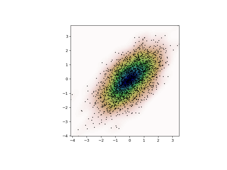
Multiscale Graph Correlation (MGC)

With multiscale_graphcorr , we can exam for independence on high dimensional and nonlinear data. Before we start, allow'southward import some useful packages:

                                >>>                                import                numpy                every bit                np                >>>                                import                matplotlib.pyplot                as                plt                ;                plt                .                style                .                utilise                (                'classic'                )                >>>                                from                scipy.stats                import                multiscale_graphcorr              

Let'due south use a custom plotting function to plot the information relationship:

                                >>>                                def                mgc_plot                (                x                ,                y                ,                sim_name                ,                mgc_dict                =                None                ,                only_viz                =                Simulated                ,                ...                                only_mgc                =                False                ):                ...                                """Plot sim and MGC-plot"""                ...                                if                not                only_mgc                :                ...                                # simulation                ...                                plt                .                figure                (                figsize                =                (                8                ,                8                ))                ...                                ax                =                plt                .                gca                ()                ...                                ax                .                set_title                (                sim_name                +                " Simulation"                ,                fontsize                =                20                )                ...                                ax                .                scatter                (                x                ,                y                )                ...                                ax                .                set_xlabel                (                'X'                ,                fontsize                =                15                )                ...                                ax                .                set_ylabel                (                'Y'                ,                fontsize                =                15                )                ...                                ax                .                axis                (                'equal'                )                ...                                ax                .                tick_params                (                axis                =                "x"                ,                labelsize                =                xv                )                ...                                ax                .                tick_params                (                axis                =                "y"                ,                labelsize                =                15                )                ...                                plt                .                show                ()                ...                                if                not                only_viz                :                ...                                # local correlation map                ...                                plt                .                figure                (                figsize                =                (                viii                ,                8                ))                ...                                ax                =                plt                .                gca                ()                ...                                mgc_map                =                mgc_dict                [                "mgc_map"                ]                ...                                # draw heatmap                ...                                ax                .                set_title                (                "Local Correlation Map"                ,                fontsize                =                xx                )                ...                                im                =                ax                .                imshow                (                mgc_map                ,                cmap                =                'YlGnBu'                )                ...                                # colorbar                ...                                cbar                =                ax                .                figure                .                colorbar                (                im                ,                ax                =                ax                )                ...                                cbar                .                ax                .                set_ylabel                (                ""                ,                rotation                =-                90                ,                va                =                "bottom"                )                ...                                ax                .                invert_yaxis                ()                ...                                # Turn spines off and create white grid.                ...                                for                edge                ,                spine                in                ax                .                spines                .                items                ():                ...                                spine                .                set_visible                (                False                )                ...                                # optimal scale                ...                                opt_scale                =                mgc_dict                [                "opt_scale"                ]                ...                                ax                .                scatter                (                opt_scale                [                0                ],                opt_scale                [                1                ],                ...                                marker                =                'Ten'                ,                s                =                200                ,                color                =                'scarlet'                )                ...                                # other formatting                ...                                ax                .                tick_params                (                bottom                =                "off"                ,                left                =                "off"                )                ...                                ax                .                set_xlabel                (                '#Neighbors for 10'                ,                fontsize                =                15                )                ...                                ax                .                set_ylabel                (                '#Neighbors for Y'                ,                fontsize                =                fifteen                )                ...                                ax                .                tick_params                (                axis                =                "ten"                ,                labelsize                =                fifteen                )                ...                                ax                .                tick_params                (                axis                =                "y"                ,                labelsize                =                xv                )                ...                                ax                .                set_xlim                (                0                ,                100                )                ...                                ax                .                set_ylim                (                0                ,                100                )                ...                                plt                .                show                ()              

Let's look at some linear data first:

                                >>>                                rng                =                np                .                random                .                default_rng                ()                >>>                                x                =                np                .                linspace                (                -                one                ,                i                ,                num                =                100                )                >>>                                y                =                x                +                0.iii                *                rng                .                random                (                x                .                size                )              

The simulation relationship can be plotted below:

                                >>>                                mgc_plot                (                ten                ,                y                ,                "Linear"                ,                only_viz                =                True                )              

../_images/mgc_plot1_01_00.png

Now, we can see the test statistic, p-value, and MGC map visualized below. The optimal scale is shown on the map as a ruddy "x":

                                >>>                                stat                ,                pvalue                ,                mgc_dict                =                multiscale_graphcorr                (                ten                ,                y                )                >>>                                print                (                "MGC examination statistic: "                ,                circular                (                stat                ,                1                ))                MGC test statistic:  1.0                >>>                                impress                (                "P-value: "                ,                round                (                pvalue                ,                1                ))                P-value:  0.0                >>>                                mgc_plot                (                10                ,                y                ,                "Linear"                ,                mgc_dict                ,                only_mgc                =                True                )              

../_images/mgc_plot2.png

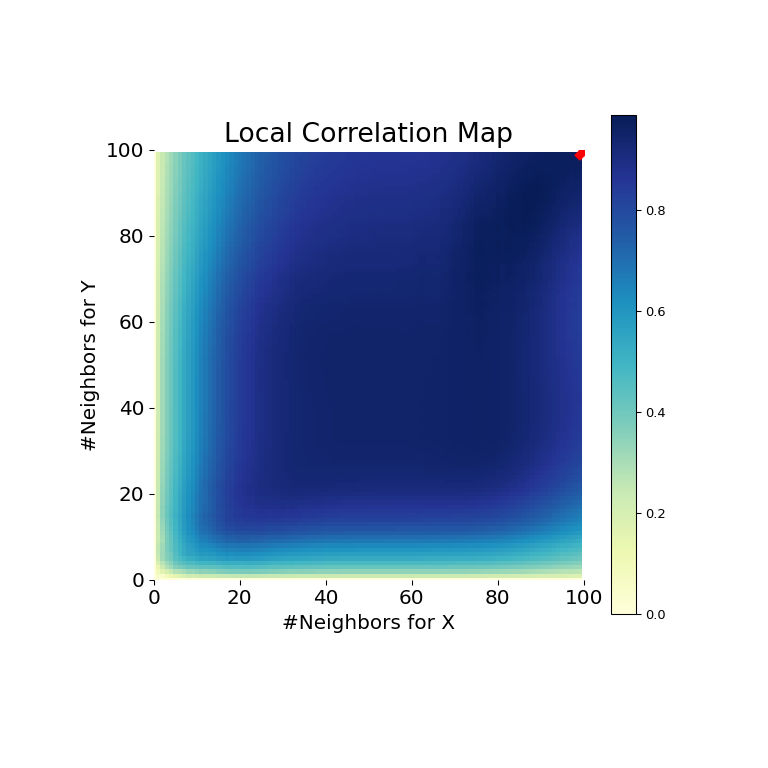
It is clear from here, that MGC is able to determine a human relationship between the input data matrices because the p-value is very low and the MGC test statistic is relatively high. The MGC-map indicates a strongly linear relationship. Intuitively, this is considering having more than neighbors will help in identifying a linear relationship between \(x\) and \(y\). The optimal scale in this case is equivalent to the global calibration, marked by a cherry spot on the map.

The same can be done for nonlinear data sets. The following \(x\) and \(y\) arrays are derived from a nonlinear simulation:

                                >>>                                unif                =                np                .                array                (                rng                .                uniform                (                0                ,                v                ,                size                =                100                ))                >>>                                10                =                unif                *                np                .                cos                (                np                .                pi                *                unif                )                >>>                                y                =                unif                *                np                .                sin                (                np                .                pi                *                unif                )                +                0.4                *                rng                .                random                (                x                .                size                )              

The simulation relationship can exist plotted beneath:

                                >>>                                mgc_plot                (                x                ,                y                ,                "Spiral"                ,                only_viz                =                True                )              

../_images/mgc_plot3_01_00.png

Now, we can see the examination statistic, p-value, and MGC map visualized below. The optimal scale is shown on the map as a cherry "x":

                                >>>                                stat                ,                pvalue                ,                mgc_dict                =                multiscale_graphcorr                (                x                ,                y                )                >>>                                print                (                "MGC examination statistic: "                ,                circular                (                stat                ,                i                ))                MGC exam statistic:  0.2  # random                >>>                                impress                (                "P-value: "                ,                circular                (                pvalue                ,                1                ))                P-value:  0.0                >>>                                mgc_plot                (                x                ,                y                ,                "Spiral"                ,                mgc_dict                ,                only_mgc                =                Truthful                )              

../_images/mgc_plot4.png

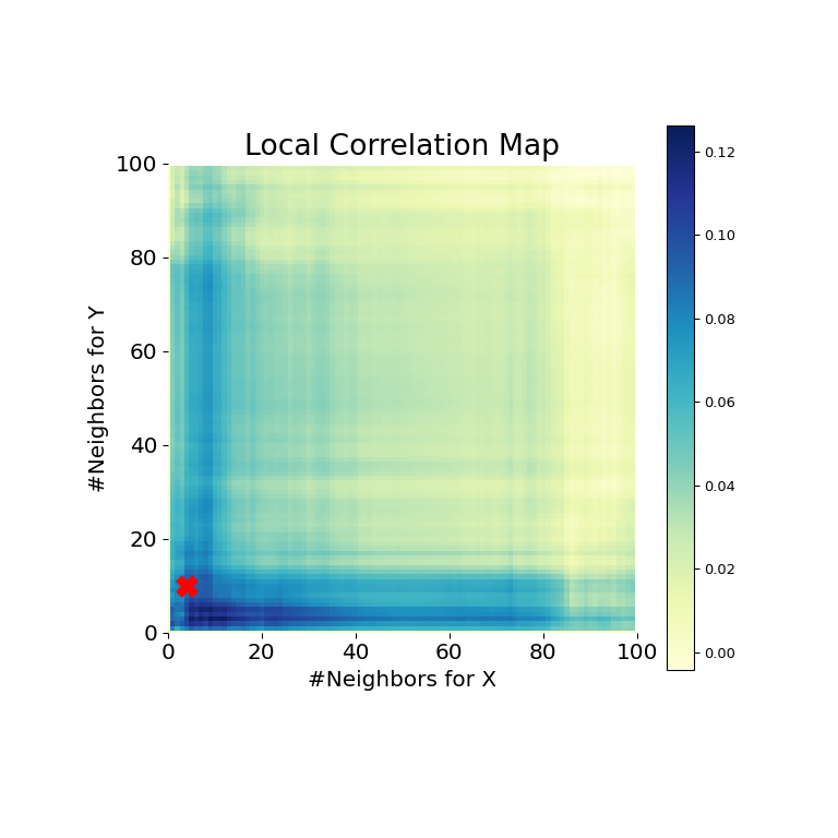
It is clear from hither, that MGC is able to determine a relationship again because the p-value is very low and the MGC test statistic is relatively high. The MGC-map indicates a strongly nonlinear relationship. The optimal scale in this case is equivalent to the local scale, marked by a ruby-red spot on the map.

Quasi-Monte Carlo

Before talking about Quasi-Monte Carlo (QMC), a quick introduction about Monte Carlo (MC). MC methods, or MC experiments, are a broad class of computational algorithms that rely on repeated random sampling to obtain numerical results. The underlying concept is to use randomness to solve problems that might exist deterministic in principle. They are oft used in physical and mathematical problems and are nigh useful when information technology is difficult or impossible to use other approaches. MC methods are mainly used in three problem classes: optimization, numerical integration, and generating draws from a probability distribution.

Generating random numbers with specific properties is a more than complex trouble than it sounds. Elementary MC methods are designed to sample points to exist independent and identically distributed (IID). Merely generating multiple sets of random points can produce radically different results.

../_images/qmc_plot_mc.png

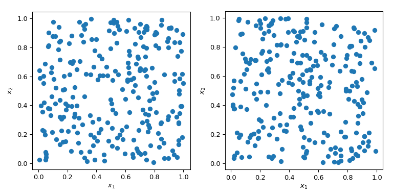
In both cases in the plot above, points are generated randomly without any knowledge about previously fatigued points. It is clear that some regions of the infinite are left unexplored - which tin can cause problems in simulations as a particular set of points might trigger a totally unlike behaviour.

A cracking do good of MC is that information technology has known convergence properties. Allow's wait at the mean of the squared sum in 5 dimensions:

\[f(\mathbf{x}) = \left( \sum_{j=ane}^{5}x_j \right)^2,\]

with \(x_j \sim \mathcal{U}(0,ane)\). Information technology has a known mean value, \(\mu = 5/3+5(5-i)/4\). Using MC sampling, we can compute that mean numerically, and the approximation error follows a theoretical rate of \(O(n^{-ane/two})\).

../_images/qmc_plot_conv_mc.png

Although the convergence is ensured, practitioners tend to want to take an exploration process which is more deterministic. With normal MC, a seed tin can exist used to have a repeatable process. But fixing the seed would interruption the convergence property: a given seed could work for a given class of problem and intermission for another i.

What is commonly washed to walk through the infinite in a deterministic manner, is to apply a regular grid spanning all parameter dimensions, also chosen a saturated design. Let'due south consider the unit-hypercube, with all premises ranging from 0 to 1. Now, having a altitude of 0.1 betwixt points, the number of points required to make full the unit of measurement interval would be 10. In a 2-dimensional hypercube the same spacing would require 100, and in 3 dimensions i,000 points. As the number of dimensions grows, the number of experiments which is required to fill the space rises exponentially equally the dimensionality of the infinite increases. This exponential growth is called "the curse of dimensionality".

                            >>>                            import              numpy              as              np              >>>                            disc              =              x              >>>                            x1              =              np              .              linspace              (              0              ,              ane              ,              disc              )              >>>                            x2              =              np              .              linspace              (              0              ,              ane              ,              disc              )              >>>                            x3              =              np              .              linspace              (              0              ,              one              ,              disc              )              >>>                            x1              ,              x2              ,              x3              =              np              .              meshgrid              (              x1              ,              x2              ,              x3              )            

../_images/qmc_plot_curse.png

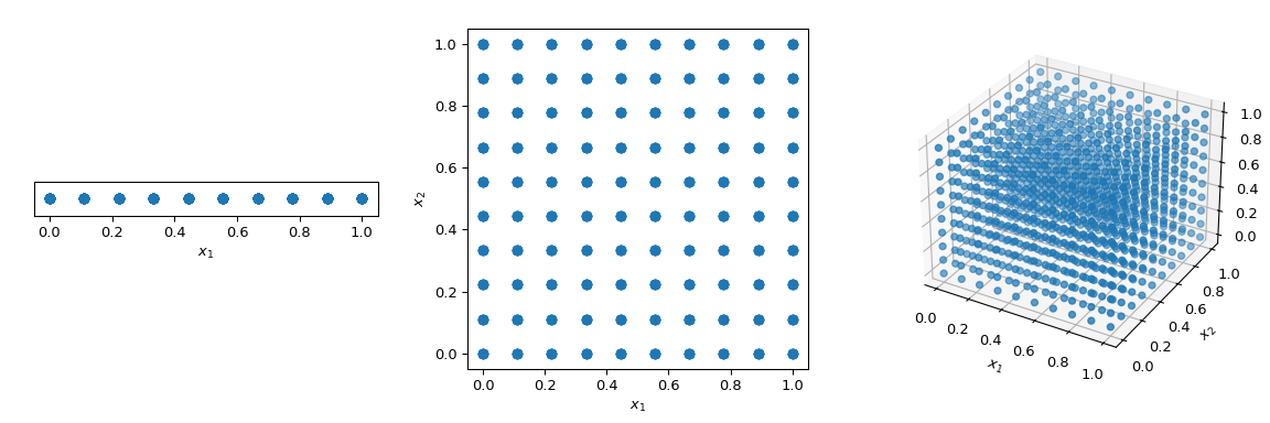
To mitigate this issue, QMC methods accept been designed. They are deterministic, take a skillful coverage of the space and some of them can be connected and retain skilful properties. The main difference with MC methods is that the points are not IID just they know virtually previous points. Hence, some methods are also referred to equally sequences.

../_images/qmc_plot_mc_qmc.png

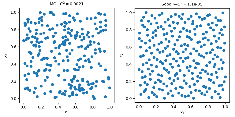
This figure presents 2 sets of 256 points. The pattern of the left is a plain MC whereas the design of the right is a QMC design using the Sobol' method. Nosotros clearly run across that the QMC version is more uniform. The points sample better near the boundaries and there are less clusters or gaps.

One mode to assess the uniformity is to use a measure chosen the discrepancy. Hither the discrepancy of Sobol' points is amend than crude MC.

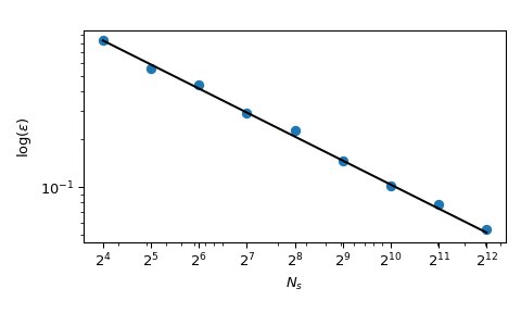
Coming back to the computation of the mean, QMC methods also have better rates of convergence for the mistake. They can achieve \(O(n^{-1})\) for this role, and even improve rates on very smooth functions. This figure shows that the Sobol' method has a rate of \(O(north^{-ane})\):

../_images/qmc_plot_conv_mc_sobol.png

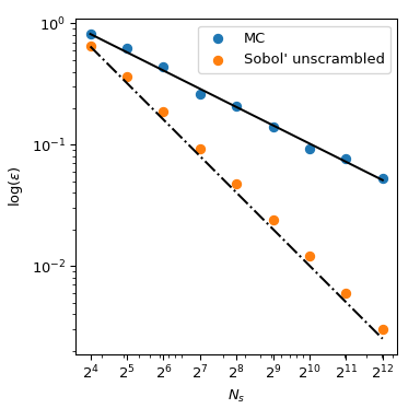
We refer to the documentation of scipy.stats.qmc for more than mathematical details.

Calculate the discrepancy

Let's consider two sets of points. From the effigy below, it is clear that the pattern on the left covers more of the space than the design on the correct. This can exist quantified using a discrepancy measure. The lower the discrepancy, the more uniform a sample is.

                                >>>                                import                numpy                equally                np                >>>                                from                scipy.stats                import                qmc                >>>                                space_1                =                np                .                array                ([[                1                ,                iii                ],                [                2                ,                6                ],                [                3                ,                two                ],                [                iv                ,                5                ],                [                v                ,                1                ],                [                6                ,                iv                ]])                >>>                                space_2                =                np                .                array                ([[                1                ,                5                ],                [                2                ,                iv                ],                [                3                ,                iii                ],                [                4                ,                two                ],                [                five                ,                i                ],                [                vi                ,                6                ]])                >>>                                l_bounds                =                [                0.5                ,                0.5                ]                >>>                                u_bounds                =                [                6.five                ,                6.5                ]                >>>                                space_1                =                qmc                .                scale                (                space_1                ,                l_bounds                ,                u_bounds                ,                reverse                =                Truthful                )                >>>                                space_2                =                qmc                .                calibration                (                space_2                ,                l_bounds                ,                u_bounds                ,                opposite                =                Truthful                )                >>>                                qmc                .                discrepancy                (                space_1                )                0.008142039609053464                >>>                                qmc                .                discrepancy                (                space_2                )                0.010456854423869011              
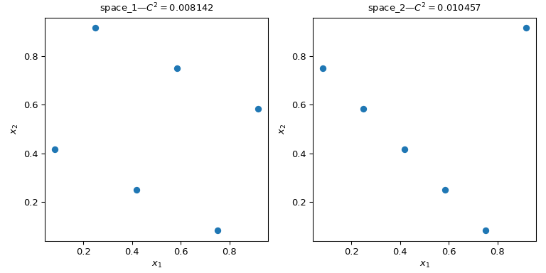
../_images/qmc_plot_discrepancy.png

Using a QMC engine

Several QMC samplers/engines are implemented. Here nosotros wait at two of the nearly used QMC methods: Sobol and Halton sequences.

                                """Sobol' and Halton sequences."""                from                scipy.stats                import                qmc                import                numpy                every bit                np                import                matplotlib.pyplot                every bit                plt                rng                =                np                .                random                .                default_rng                ()                n_sample                =                256                dim                =                ii                sample                =                {}                # Sobol'                engine                =                qmc                .                Sobol                (                d                =                dim                ,                seed                =                rng                )                sample                [                "Sobol'"                ]                =                engine                .                random                (                n_sample                )                # Halton                engine                =                qmc                .                Halton                (                d                =                dim                ,                seed                =                rng                )                sample                [                "Halton"                ]                =                engine                .                random                (                n_sample                )                fig                ,                axs                =                plt                .                subplots                (                1                ,                2                ,                figsize                =                (                8                ,                iv                ))                for                i                ,                kind                in                enumerate                (                sample                ):                axs                [                i                ]                .                scatter                (                sample                [                kind                ][:,                0                ],                sample                [                kind                ][:,                1                ])                axs                [                i                ]                .                set_aspect                (                'equal'                )                axs                [                i                ]                .                set_xlabel                (                r                '$x_1$'                )                axs                [                i                ]                .                set_ylabel                (                r                '$x_2$'                )                axs                [                i                ]                .                set_title                (                f                '                {                kind                }                —$C^2 = $                {                qmc                .                discrepancy                (                sample                [                kind                ])                :                .2                }                '                )                plt                .                tight_layout                ()                plt                .                show                ()              
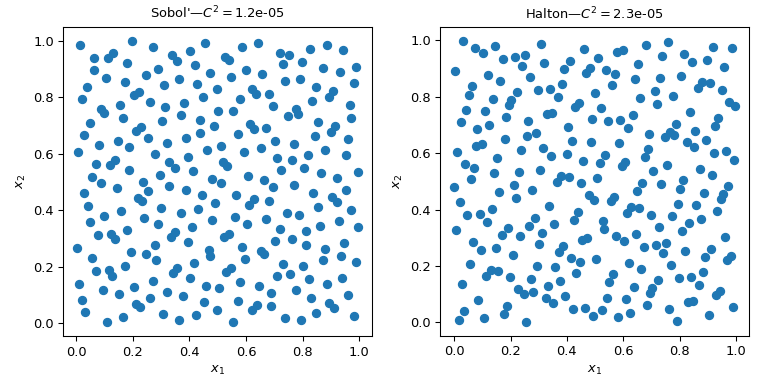
../_images/qmc_plot_sobol_halton.png

Warning

QMC methods require detail care and the user must read the documentation to avoid mutual pitfalls. Sobol' for instance requires a number of points post-obit a power of two. As well, thinning, burning or other point pick tin break the backdrop of the sequence and result in a set of points which would non exist ameliorate than MC.

QMC engines are state-aware. Pregnant that you lot can go on the sequence, skip some points, or reset it. Permit's take five points from Halton . And then enquire for a 2d ready of v points:

                                >>>                                from                scipy.stats                import                qmc                >>>                                engine                =                qmc                .                Halton                (                d                =                2                )                >>>                                engine                .                random                (                5                )                array([[0.22166437, 0.07980522],  # random                                  [0.72166437, 0.93165708],                                  [0.47166437, 0.41313856],                                  [0.97166437, 0.19091633],                                  [0.01853937, 0.74647189]])                >>>                                engine                .                random                (                v                )                array([[0.51853937, 0.52424967],  # random                                  [0.26853937, 0.30202745],                                  [0.76853937, 0.857583  ],                                  [0.14353937, 0.63536078],                                  [0.64353937, 0.01807683]])              

Now nosotros reset the sequence. Request for 5 points leads to the aforementioned first v points:

                                >>>                                engine                .                reset                ()                >>>                                engine                .                random                (                5                )                array([[0.22166437, 0.07980522],  # random                                  [0.72166437, 0.93165708],                                  [0.47166437, 0.41313856],                                  [0.97166437, 0.19091633],                                  [0.01853937, 0.74647189]])              

And here we accelerate the sequence to go the aforementioned 2d set of 5 points:

                                >>>                                engine                .                reset                ()                >>>                                engine                .                fast_forward                (                5                )                >>>                                engine                .                random                (                v                )                array([[0.51853937, 0.52424967],  # random                                  [0.26853937, 0.30202745],                                  [0.76853937, 0.857583  ],                                  [0.14353937, 0.63536078],                                  [0.64353937, 0.01807683]])              

Note

By default, both Sobol and Halton are scrambled. The convergence properties are better, and information technology prevents the appearance of fringes or noticeable patterns of points in high dimensions. There should be no practical reason non to utilise the scrambled version.

Making a QMC engine, i.e., subclassing QMCEngine

To make your own QMCEngine , a few methods have to be divers. Following is an example wrapping numpy.random.Generator .

                                >>>                                import                numpy                every bit                np                >>>                                from                scipy.stats                import                qmc                >>>                                class                RandomEngine                (                qmc                .                QMCEngine                ):                ...                                def                __init__                (                self                ,                d                ,                seed                =                None                ):                ...                                super                ()                .                __init__                (                d                =                d                ,                seed                =                seed                )                ...                                self                .                rng                =                np                .                random                .                default_rng                (                self                .                rng_seed                )                ...                ...                ...                                def                random                (                self                ,                n                =                one                ):                ...                                self                .                num_generated                +=                n                ...                                return                self                .                rng                .                random                ((                n                ,                self                .                d                ))                ...                ...                ...                                def                reset                (                self                ):                ...                                self                .                rng                =                np                .                random                .                default_rng                (                self                .                rng_seed                )                ...                                cocky                .                num_generated                =                0                ...                                return                self                ...                ...                ...                                def                fast_forward                (                cocky                ,                north                ):                ...                                self                .                random                (                n                )                ...                                return                self              

Then we use information technology as whatsoever other QMC engine:

                                >>>                                engine                =                RandomEngine                (                2                )                >>>                                engine                .                random                (                5                )                array([[0.22733602, 0.31675834],  # random                                  [0.79736546, 0.67625467],                                  [0.39110955, 0.33281393],                                  [0.59830875, 0.18673419],                                  [0.67275604, 0.94180287]])                >>>                                engine                .                reset                ()                >>>                                engine                .                random                (                v                )                array([[0.22733602, 0.31675834],  # random                                  [0.79736546, 0.67625467],                                  [0.39110955, 0.33281393],                                  [0.59830875, 0.18673419],                                  [0.67275604, 0.94180287]])              

Guidelines on using QMC

  • QMC has rules! Be sure to read the documentation or you might take no benefit over MC.

  • Use Sobol if you need exactly \(2^one thousand\) points.

  • Halton allows to sample, or skip, an arbitrary number of points. This is at the price of a slower rate of convergence than Sobol'.

  • Never remove the get-go points of the sequence. Information technology will destroy the properties.

  • Scrambling is always better.

  • If you use LHS based methods, you cannot add points without losing the LHS backdrop. (There are some methods to do and so, but this is not implemented.)

perezancentiond.blogspot.com

Source: https://docs.scipy.org/doc/scipy/tutorial/stats.html

0 Response to "how to find what is the distribution of an attribute python"

إرسال تعليق

Iklan Atas Artikel

Iklan Tengah Artikel 1

Iklan Tengah Artikel 2

Iklan Bawah Artikel